Machine Learning Basics

Machine Learning is the field of study that gives computer the ability to learn without being explicitly programmed. A computer program is said to learn from experience E with respect ot some task T and some performance measure P, if its performance on T , as measured by P, improves with experience E.
Machine Learning Algorithms:

1. Supervised Learning
   • Regression (continuous output)
   • Classification (discrete valued output)
2. Unsupervised Learning

Linear Regression

Linear Regression with one variable

$Hypothesis : h_{\theta}(x) = \theta_{0} + \theta_{1}x$
$Parameters : \theta_{0}, \theta_{1}$
$Cost function : J(\theta_{0}, \theta_{1}) = \frac{1}{2m}\sum\limits_{i=1}^{m}(h_{\theta}(x^{i}) - y^{i})^2$
$Goal : Minimize : J(\theta_{0},\theta_{1})$

Gradient descent
Repeat until covergence
$\theta_{j} := \theta_{j} - \alpha\frac{\partial}{\partial\theta_{j}}J(\theta_{0}, \theta_{1})$ (for j=0 and 1)

$\theta_{0} := \theta_{0} - \alpha\frac{1}{m}\sum\limits_{i=1}^{m}(h_{\theta}(x^{i}) - y^{i})$

$\theta_{1} := \theta_{1} - \alpha\frac{1}{m}\sum\limits_{i=1}^{m}(h_{\theta}(x^{i}) - y^{i})x^{i}$

Linear Regression with multiple variable

$Hypothesis : h_{\theta} = \theta^{T}x = \theta_{0}x_{0} + \theta_{1}x_{1} + . . . \theta_{n}x_{n}$

$Parameters : \theta = [ \theta_{0}, \theta_{1}, \theta_{2}, . . \theta_{n} ]^T$

$Cost function : J(\theta) = \frac{1}{2m}\sum\limits_{i=1}^{m}(h_{\theta}(x^{i}) - y^{i})^2$

Gradient descent
Repeat until convergence
$\theta_{j} := \theta_{j} - \alpha\frac{\partial}{\partial\theta_{j}}J(\theta)$ (simultaneously update for every j=0,1,2...n)

$\theta_{j} := \theta_{j} - \alpha\frac{1}{m}\sum\limits_{i=1}^{m}(h_{\theta}(x^{i}) - y^{i})x^{j}$

Method to solve of $\theta$ analytically : Normal Equation

Let $h_{\theta} = \theta^{T}x = \theta_{0}x_{0} + \theta_{1}x_{1} + . . . \theta_{n}x_{n}$

$\implies (\theta^Tx)^T = Y$

$\implies x\theta^T = Y$

$\implies x^Tx\theta^T = x^TY$

$\implies \theta^T = (x^Tx)^{-1}x^TY$

Logistic Regression

In Logistic regression, $0 \le h(\theta) \le 1$
In Linear regression, $h(\theta) = \theta^Tx \in (R)$
In Logistic regression, $h(\theta) = g(\theta^Tx)$
where,
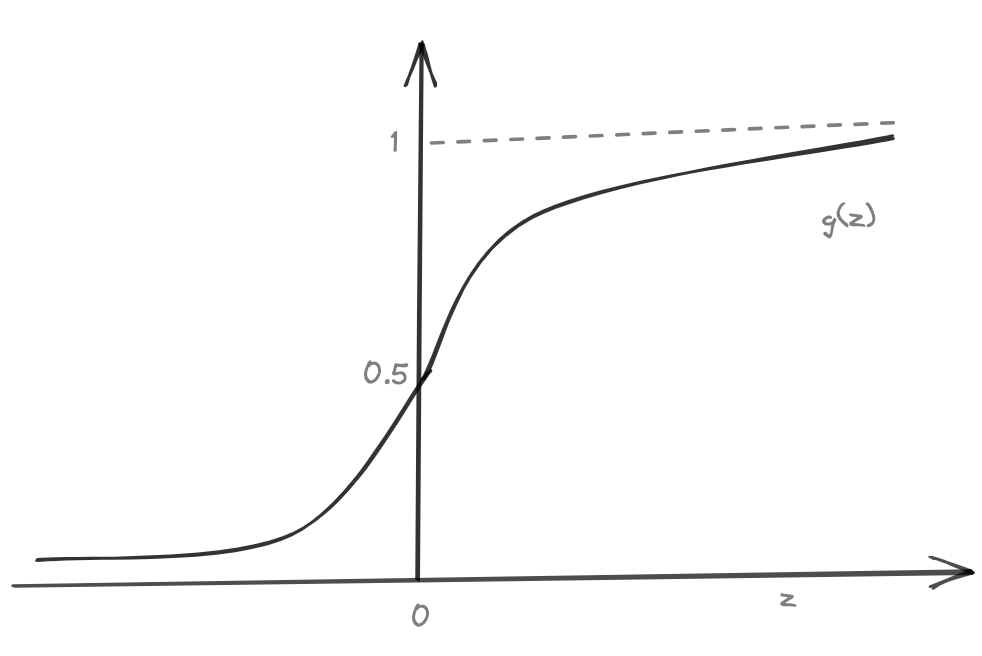
$\ \ \ \ \ \ \ g(z) = \frac{1}{1 + e^{-z}} = sigmoid/logistic function$

$\implies h_{\theta}(x) = \frac{1}{1 + e^{-\theta^Tx}}$

$h_{\theta}(x)$ = estimated probability that y=1 on input x. i.e., $h_{\theta}(x) = P(y=1|x;\theta)$ = prob. that y=1, given x, parametrized by $\theta$. Now; $h_{\theta}(x) = 0.5$

$\implies \frac{1}{1 + e^{-\theta^Tx}} = 0.5$

$\implies \theta^Tx = 0$

so, $h_{\theta}(x) \ge 0.5 \implies \theta^Tx \ge 0$ and, $h_{\theta}(x) \le 0.5 \implies \theta^Tx \le 0$

Ex. Let $h_{\theta}(x) = g(\theta_{0} + \theta_{1}x_{1} + \theta_{2}x_{2}) = g(\theta^Tx)$ (at $\theta=[-3,1,1]$)
$\implies Predict \ y if \ -3 + x_1 + x_2 \ge 0$
$\implies x_1 + x_2 \ge 3$ (Linear decision boundary)

Cost function for logistic regression
$J(\theta) = -\frac{1}{m}\sum\limits_{i=1}^{m}[y^{i}log(h(x^{i},\theta)) + (1-y^{i})log(1-h(x^{i},\theta))]$

Following to to be completed . . .

Multi-class Classification

Neural Networks

Machine Learning Diagnostics